Gephi Training (RMCLAS 2015)

Here are your data sets and links to the programs needed for today’s workshop:

Gephi

Palladio

Open Refine

Data Sets from Google Drive

Teaching with Tumblr and StoryMapJS

Another semester yielded another crop of impressive DH projects in my courses on the history of Colonial Latin America and the History of Mexico. Utilizing Tumblr for the first time in my Colonial Latin America course (HIST 410), students were given free rein to create a visual project centered on a topic of their choice pulled from within the chronological and geographic boundaries of the course. Selecting the top five Tumblrs from this course was EXTREMELY difficult as my students produced some amazing work product, but here are the top 5 projects:

Women of Colonial Latin America

A Cartographic Analysis of Colonial Latin America

Slavery: Conditions in Colonial Latin America

Racialized Depictions of Women & Children

The Chronicle of Felipe Guaman Poma de Ayala

For the first time in my History of Mexico course (HIST 412), my students used StoryMapJS to produce highly visual, geospatial historical narratives on a topic of their choice. Here are the top 3 projects:

The Mexican-American War

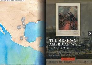
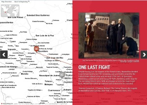
The French Intervention in Mexico

Afro-Mexicans: An Invisible Population

Minus some minor errors in proper citations, the formatting of those citations, and the use of non-academic sources for images (I’m looking at you Wikimedia Commons), the majority of projects across both classes were of very high quality. Students greatly enjoyed (or so they told me) working on these projects during the course of the semester and the projects provided an excellent opportunity to hone their abilities to produce well-researched, well-documented, highly accessible, and highly engaging historical narratives. Additionally, I believe that this kind of work product can and should be a prominent part of students’ portfolios when applying for graduate school, internships, and jobs, as the skills acquired from this hands-on, project-based approach to learning provides my students with the knowledge necessary to take their passion for history into the digital realm of the 21st century.

Tutorial on Juxtaposing Historical & Modern Images

Encouraged and inspired by my colleague Diana Montaño and Clayton Kauzlaric’s “Then & Again” project, I tried my hand at juxtaposing vintage, historical images onto modern ones. This approach, which visualizes physical changes over time, creates a powerful connection between the past and present of a particular place. In this tutorial, I will introduce the basic methodology for creating such an image using free, nearly universally-available tools. However, keep in mind that I am very much a novice at image retouching and editing, and feedback is much appreciated as I continue to improve this process and its end products.

Tools used:

Google Maps, Gimp 2.8, Microsoft Office Picture Manager, Microsoft Paint (seriously)

Steps:

1. Locate the historical image you wish to superimpose onto a modern one. For this example, I will be utilizing the fantastic digital archive of historical photographs of Mexico City created by Carlos Villasana, Juan Carlos Briones, and Rodrigo Hidalgo and located on their Facebook page, La ciudad de Mexico en el tiempo.

2. In this case, I selected a photograph of the iconic Palacio de Bellas Artes under construction during the first decades of the twentieth century (See below). Once one has decided on the historical image, it’s time to find its modern counterpart using Google Maps.

3. Normally, one would need to open up a browser, go to the Google Maps site, and locate the approximate modern location of your historical object/building/event from the vintage photograph. Fortunately for those of us interested in the history of Mexico City, La ciudad de Mexico en el tiempo’s photo galleries include links directly to the Google Maps Street View corresponding to the vintage images. (See image below.)

4. While viewing the modern location In Google Maps Street View, attempt to recreate the same angle and viewing distance as the original historical image. This can be frustrating as Street View may not provide the perfect perspective for the juxtaposition of the two images. This issue can be resolved by taking one’s own photograph at the physical location, but of course this is much more time-consuming and may require some travel. Once you have lined up your perspective in Street View as best as possible, it’s time to capture the images.

5. To capture the two images (historical & modern) for beginning the juxtaposition process, I’ll use one method for both images, although there are several ways to accomplish this step. For all images that cannot be right-clicked on and the image directly downloaded, you can use the “print screen” button on your keyboard. Move your mouse cursor away from the area of the image you want to capture and click the print screen button once. (See image below.)

6. This single press of the button copies the entirety of your screen to be pasted into an image retouching program, which in this case, will be good old Microsoft Paint. Open up Paint and press the “paste” icon in the upper left corner of the program. (See image below.)

7. Once you’ve hit this button, the captured image should be pasted into Paint for capture as a .jpeg file. Go to the drop down icon in the upper-left corner of the program and select “Save as” and then “JPEG picture.” (See image below.)

8. Do this process twice, once for the Street View image and one for the historical image, and save your new image files to a secure, familiar location on your hard drive (these steps can be skipped if you scanned and/or uploaded the image files to your hard drive yourself rather than from the web).

9. To edit these images for juxtaposition, we’ll need to crop them down a bit, so open these two image files with Microsoft Office Picture Manager or your image editor of choice. You can select which program to open these files with by right-clicking on the image file and selecting the program from the drop-down list. Once you’ve opened the image file, you’ll want to open up the option to “edit pictures” or its equivalent. (See image below.)

10. To crop out the unwanted content surrounding the images, use the “crop” tool to edit the image. (See image below.)

11. Once this has been done, the perspective of the modern image should resemble the historical image as closely as possible. (See image below.)

12. Now that we have our two images looking as similar as possible prior to juxtaposing, we are ready to open up the modern image first using our free image retouching program, GIMP. Certainly it is possible to retouch these photos using Adobe Photoshop, but money doesn’t grow on trees, and as an adjunct professor I’m always looking for ways to cut costs and instead utilize good quality freeware. Download and install GIMP (I’ll be using GIMP 2.8 here) from their official website.

13. Open the modern image pulled from Street View first, clicking on the “open” tab found under the “File” icon. (See image below.)

14. Once you’ve successfully imported the image into GIMP, it should look like the image below. A multitude of tools are now at your disposal for image retouching, but first you need to import the historical image (See image below.)

15. Instead of using “open” to bring in the historical image, go to “File,” select “Open as Layers,” and then the image file for the historical photograph. (See image below.)

16. Once you’ve imported the historical image in as a separate layer, your screen in GIMP should look like the image below. Now it’s time to manipulate the size and positioning of the historical image to match the modern image. (See image below.)

17. The first tool needed to manipulate the historical image is the “move” tool, located in the “toolbox” window on the left side of the program. This tool allows you to grab and relocate the positioning of the historical image atop the modern one. (See image below.)

18. The other very important tool utilized for this process is the “scale” tool, also located in the left-hand toolbox window. This tool allows you to resize the proportions of the historical image to fit as precisely as possible on top of the proportions of the modern image. (See image below.)

19. After you click the scale tool button, left click on the historical image to begin resizing it. A grid and resizing boxes will appear over the historical image, allowing you to either input the exact pixel dimensions of the image or to left click and hold on the resizing boxes at the edges of the image.(See image below.) I prefer to resize using the latter method, but be sure to hit the “scale” button on the pop-up box once your resizing process is complete. However, to “perfectly” line up the two images, you’ll need to use a combination of “scale,” “move,” and a particular image attribute explained in the next step.

20. The obvious challenge in lining these two images up and resizing/repositioning the historical image is the inability to see through the historical to the modern for accurate juxtaposition. This can be resolved by adjusting the “opacity” of the historical image via a slider bar located under the “Layers” window on the right side of the screen. (See image below.) By clicking/sliding this attribute’s value (0-100), the historical image becomes more transparent as the opacity value goes down. By doing this, the modern image can more easily be seen in the background, allowing for accurate resizing/positioning of the historical image.

21. As you reposition and resize your historical image, be sure to use visual reference points in your two images to ensure proper overlap. In this example, I used three specific visual markers. (See image below.)

22. Once the two images are properly juxtaposed on top of one another (see image below), it’s time to remove unwanted visuals from around the historical image in order to blend it into the modern landscape.

23. The final tool to be utilized is the “eraser” tool, located on the toolbox window on the left side of the program. (See image below.) Adjust your brush size, hardness, and opacity to remove the background from the historical image.

24. Carefully use the eraser tool to remove unwanted image materials around the historical image, careful not to go too quickly or with a brush that is too large to preserve the fine details at the edge of the building. (See image below.)

25. This process of erasing and blending is where an artistic eye can be helpful, as the best means of blending in the street lamps, bushes, and pedestrians to appear as a natural part of this hybrid image is up to the editor. Use a medium-opacity eraser at the edges of the historical image to carefully blend it into the modern background to complete the juxtaposing process. (See image below.)

26. You can now finalize your juxtaposed image by exporting it from the program. Click the file icon and select “export” from the drop down menu. You can select the file type (.png, .jpeg, etc.) and save location, click the export button, and you are done! (See image below.)

27. These steps are a very crude, simple means of juxtaposing a historical and modern image, but I hope this tutorial provides a starting point for historical enthusiasts/image retouching novices to get started. I will continue to update and edit this tutorial as I learn more about fine tuning the process and improving the quality of the final product. I look forward to seeing your images!

Teaching with Interactive Timelines via Tiki-Toki

After the wonderful but time-intensive relationship with Twitter in my world history surveys last semester, I decided to take a break from group projects and social media. This semester I gave my students a chance to create their own uncompromising, individual vision for a history project. Using the free, web-based software provided by Tiki-Toki, my 260+ students all “translated” research papers they completed earlier in the semester into digital, interactive timelines available for public consumption. As I stated in my post concerning the Twitter project, I am a huge believer in the capacity for these types of digital projects to empower, inspire, and educate students through the use of such a student-centered approach to learning. Through the creation of these timelines, students learn a greater appreciation of chronology and periodization, the art of constructing a historical narrative fit for “everyman” usage, and training in the usage of a powerful digital toolkit. I’m happy to say it was extremely difficult to narrow it down, but below are the top ten timelines produced by my students this semester.  Enjoy!

The Plague of Ancient Athens

The Battle of Gettysburg

The Start of the French Revolution

The Atomic Bombing of Hiroshima & Nagasaki

The Winter War

The Punic Wars: How Rome Conquered the Mediterranean

Prostitution in 18th & 19th-century France

The Spanish Flu

Eisenhower’s National Interstate and Defense Highway

Jack the Ripper: A Social Construct

If These Bones Could Tweet: Teaching Introductory-Level History Courses with Twitter

As I transitioned from student to professor over the last year, I sought to find ways to transform the passive, top-down, large-scale lecture course into a student-centered, highly active, and goal-oriented collaborative learning environment.  To accomplish this, I have come up with an introductory-level course build utilizing Twitter and Google Drive in order to re-imagine the concept of the in-class “group project.”  In my three introductory-level world history courses this semester involving the participation of over 325 students, large-scale, collaborative group projects designed to “put history into action” serve as the central research project for each class.  The students, primarily freshman, have formed groups of 10-15 individuals tasked with the goal of a producing and publishing a work of digital public history via Twitter over the course of the semester.  I certainly remain skeptical of the promotion of technology in the classroom as the cure-all for the ills of higher education, but having seen the impact of this digital project on my students even within the short span of the first seven weeks of the semester, I have become a true believer in the potential of social media as a powerful pedagogical tool for transforming students into active, passionate learners working within these new “communities of practice.”

During the course of the semester, these groups work collectively to identify potential primary and secondary sources on a given historical topic, analyze those sources, compile data gleaned from those sources into a digital database stored on Google Drive, and finally publish a collaboratively-produced historical narrative using Twitter’s micro-blogging service, complete with metadata in the form of hash tags.  Through the merger of traditional historical methodologies with what was formerly a social media platform employed by students for “idle use,” Twitter is transformed into a powerful tool for turning students into producers, rather than mere consumers, of historical knowledge.  This hands-on engagement with historical sources and the utilization of social media, web publication, and digital databases to create collaborative, digital public history projects democratizes the practice of history and expands the notion of public history from exhibits and programs created for public viewing to an interactive historical space shared by its student creators and interested members of the public.

In the recent past, a number of educators have used social media such as Twitter as a means of extending student discussion outside the physical confines of the classroom.  My experiment attempts to go one step further towards integrating social media into the classroom by making it the central focus of the course itself.  These student-led Twitter projects form the pedagogical core of my world history courses and  provide instruction and practice in historical methodology, including the construction and manipulation of historical databases, navigating historical archives and databases, the analysis of primary and secondary sources, and the art of writing historical narratives.  Looking to the high-quality examples of historical publication on Twitter such as @RealTimeWW2, @TitanicRealTime/@WChapelRealTime, @CryForByzantium, and numerous others, these student-led projects seek to contribute to the body of historical knowledge available online.

Learning outcomes from this process are numerous and varied: students quickly learn to discern an academic from a non-academic source; work collectively to determine the best narrative structure for the publication of their particular topic; develop an awareness of the opportunities and challenges inherent to communicating information through digital media; utilize digital and physical library resources; construct Chicago Manual of Style-formatted bibliographies for their sources; and become “knowledgeable users” of several digital technologies.  Additionally, this project presents a powerful opportunity for “deep learning” on their historical topic, helping to offset the rapid pace of introductory-level courses which often are forced to skim the surface  of historical knowledge to stay on schedule.  The flexible, student-centered nature of this project also allows students to express their creativity and diverse personal perspectives, as a significant proportion of the projects being developed this semester deal with some aspect of gender, race, and/or class.

As of November 1st, the majority of groups have “gone live” and are now publishing their content on Twitter, allowing me to finally reveal the results of my students’ hard work over the last eight weeks.  They will continue publishing for the remaining six weeks of the semester, allowing their accounts to roll out at a semi-reasonable pace and hopefully attracting some interest from you, the public.  Are these projects perfect?  Absolutely not.  There will be some errors, as with any endeavor of this size created at such a high rate of speed, things will still slip through the cracks during the final edits.  However, while I am concerned with the historical accuracy and presentation of these topics, I am much more concerned with what my students have learned during the process of researching, writing, and synthesizing historical information for their projects.

I could not be happier with the ways in which this concept-driven, interactive course format has motivated and excited my students beyond what I’ve ever experienced before.  Innumerable students have approached me outside the classroom to express how enthusiastic they are about this project and how they have shared their work on the project with a family member, their friends, and even potential employers.  Additionally, this project allows exceptional students to stand out from their peers in a number of ways which traditional assessments simply do not allow for.  The leadership skills, drive, and creativity demonstrated by many of my first-semester freshmen has changed my (and I think their) assumptions about the complexity of tasks they are capable of successfully completing.

This kind of public, immersive digital project produces an end product which students are extremely proud of, as they are helping to contribute to the growing body of historical knowledge available on the web.  I believe these kinds of innovative digital projects could play a significant role in the future of the historical practice and directly address the concerns expressed in a recent article in Perspectives in History written by 2012 National Humanities Medal recipient Edward L. Ayers, in which he describes his undergraduate students’ appeal for historians “to engage people where they are…we must employ the tools people use every day to build communities of understanding in real time…[and] expand our definition of scholarship so that it would flourish in the new world of social media. [The students] felt certain that the public that would be interested in what scholars were writing if they could just see it. They wanted to put scholarship to work in the world, to make it a living presence.”[1]

For my future teaching, there is no going back to purely traditional methods.  As early as this spring, I plan to experiment with a number of other digital tools in my introductory-level courses, including the creation of interactive map layers utilizing Google Earth, virtual museum exhibits using Omeka/Neatline, and visual narratives constructed using Tumblr.  Also, this spring I have the honor of teaching the first upper-division methods course on the practice of digital history ever offered at Colorado State University, so next semester be prepared for a flurry of online tutorials and blog posts referencing our work across a number of my courses (you can follow me on Twitter at @rjordan_csu to stay on top of all my updates.)  For our Twitter projects for this semester, the following is a comprehensive list of accounts if you’re interested in viewing my students’ work and to start following them:

HIST 170.001 – World History: Ancient to 1500 (Topics on the Mediterranean World):

• @Gladiator_Facts – A historical exploration of the lives of gladiators in ancient Rome.
• @lifeofcleopatra – The life and reign of Cleopatra VII of Egypt, one of the most famous and fascinating women of the ancient world.
• @AncientSports – A historical exploration of the variety of sports played in the ancient Greek world (GSPN).
• @CenturionDaily – The life and times of a Roman centurion in the time of the Roman Civil War.
• @Apostle__Paul – A historical account of the life and world of the Apostle Paul.
• @Techno_Rome – A historical exploration of the technologies introduced and employed during the time of the Roman Empire.
• @CaligulaTheMad – The life and reign of Caligula, one of the most infamous Roman emperors of all time.

HIST 171.004 – World History: 1500 to Present (Topics on the Industrial Revolution):

• @WomenatWork171 – The narrative of the lives of four women living in London, England during the Industrial Revolution.
• @VoicesofBedlam – A historical narrative describing the lives and conditions of Bethlem Mental Institution in the 19th century.
• @LawandOrderVL – Two fictional detectives solve real cases straight from the criminal underworld of 19th-century London.
• @RailroadsMuseum – A historical examination of the development of railroads on a global scale.
• @TheOilBoomer – A historical narrative of the life of John D. Rockefeller and the oil empire he created.
• @LondonLaborers – A historical retelling of the lives of child laborers in London during the Industrial Revolution.
• @FivePoints_NYC – A historical narrative of the multitude of people living in the infamous Manhattan neighborhood known as Five Points during the 19th century.
• @Allanpinkerton3 – Historical facts and stories involving the Pinkerton Agency.
• @MedicinalRevo – A historical examination of aspects of medicine during the Industrial Revolution.
• @londonunderworl – A narrative of the lives of everyday people living in London, England during the Industrial Revolution.

HIST 171.006 – World History: 1500 to Present (Topics on World War II):

• @atomiclibrary – Facts and historical fiction pertaining to the Manhattan Project and the development of the first nuclear weapons.
• @battleofmoscow – The devastating Battle of Moscow and events leading up to this military struggle from various perspectives.
• @GoForBroke_442 –  The stories of the fighting men of the U.S. Army’s 442nd Battalion during their distinguished service in World War II.
• @Story_AnneFrank – A historical exploration of the world of Anne Frank and her diary.
• @thebritblitz – A historical examination of the Nazi bombing campaign on London during World War II.
• @ww2propaganda – The history of World War II as told through a collection of global war propaganda.
• @OpWatchtower – A livetweeting of the Naval Battle of Guadalcanal and Operation Watchtower from the perspective of a fictional embedded journalist.
• @StalingradWW2 – A historical retelling and examination of the Soviet counterattack codenamed “Operation Uranus” centered on the city of Stalingrad from November 19-23, 1942.  (Live tweets to come).
• @WWIIPearlHarbor – A historical retelling and examination of the events of December 7, 1941, “a date which will live in infamy.” (This group will be doing some major live tweeting later in the semester).

---

[1] Edward L. Ayers, “An Assignment from Our Students: An Undergraduate View of the Historical Profession,” Perspectives in History, September 2013, accessed October 8, 2013, http://bit.ly/18O7fPK.

My “Master List” of Digital Humanities Centers/Projects/Initiatives (US only)

In an attempt to answer a question frequently asked on Twitter: “What universities have graduate programs in the digital humanities?” I offer up this latest post.  As of now, there is no “master list” of universities offering digital humanities courses at either the undergraduate or graduate level, provoking me to produce my own list of such programs.  However, as much as I believe my initial attempt to answer this question is a step in the right direction, it heavily relies upon a certain assumption.  My undoubtedly incomplete list found below is composed of DH centers, projects, and initiatives at a number of universities in the United States.  Considering that these universities have devoted substantial financial and intellectual resources to the study of the digital humanities, I assume that they also are offering courses on the subject as part of their regular curriculum.  Certainly @DHcenterNet’s list of digital humanities centers is a good place to start, but at the time of this post, the following serves as a more comprehensive list (please feel free to email me at r.jordan@colostate.edu to add additional universities to this list or to correct any of the information found below):

Alabama Digital Humanities Center at the University of Alabama

Baker-Nord Center for the Humanities at Case Western Reserve University

CATH: Center for Applied Technologies in the Humanities at Virginia Tech University

CDH: Center for Digital Humanities at the University of South Carolina

CDRH: Center for Digital Research in the Humanities at the University of Nebraska-Lincoln

Center for Digital Humanities and Culture at the Indiana University of Pennsylvania

Center for Digital Humanities at Brock University

Center for Digital Scholarship at Brown University

Center for Scholarly Communication & Digital Curation at Northwestern University

Centre for Oral History and Digital Storytelling at Concordia University

CHNM: Center for History and New Media at George Mason University

CMS: Comparative Media Studies at Massachusetts Institute of Technology

CPHDH: Center for Public History + Digital Humanities at Cleveland State University

CTSDH: Center for Textual Studies and Digital Humanities at Loyola University

CUNY Digital Humanities Initiative (all 24 CUNY campuses)

DHC: Digital Humanities Center at Columbia University

DHI: Digital Humanities Initiative at Hamilton College

Digital History Lab at California State University-San Marcos

Digital History Lab at Harvard University

Digital History Lab at Princeton University

Digital History Lab at the University of Massachusetts-Amherst

Digital Humanities 2.0 Collaborative at the University of Minnesota

Digital Humanities Initiative at Hamilton College

Digital Innovation Lab at the University of North Carolina

Digital Scholarship Commons at Emory University

Digital Scholarship Lab at the University of Richmond

Digital Studio for Public Humanities at the University of Iowa

DSC: Digital Scholarship Center at the University of Oregon

HASTAC: Humanities, Arts, Science, and Technology Advanced Collaboratory at Duke University

Humanities Research Center at Rice University

Humanities Technology and Research Support Center at Brigham Young University

I-CHASS: Institute for Computing in the Humanities, Arts, and Social Science at the University of Illinois

IDAH: Institute for Digital Research in the Humanities at the University of Kansas

IDHMC: Initiative for Digital Humanities, Media, and Culture at Texas A&M University

Institute for Advanced Technology in the Humanities at the University of Virginia

Interdisciplinary Humanities Research Center, University of Delaware

IRIS: Interdisciplinary Research and Informatics Scholarship Center at Southern Illinois University

MATRIX: Center for Humane, Arts, Letters, and Sciences Online at Michigan State University

MITH: Maryland Institute for Technology in the Humanities at the University of Maryland

Research in Computing for the Humanities at the University of Kentucky

SJCDH: South Jersey Center for Digital Humanities at Stockton College

Spatial History Project at Stanford University

Virginia Center for Digital History at the University of Virginia

Wired Humanities Project at the University of Oregon

Getting started with Gephi

For this post, I’m going to provide step-by-step instruction for those of you interested in creating network graphs using Gephi.  Certainly there is other open-source software available for visualizing social network and textual data such as Pajek (this website could use a serious design update), but at the time of this post, Gephi 0.8.2-beta has some significant advantages.  Software such as Pajek allows you to save your project file as a .bmp, .png, or .svg, but Gephi allows you to save your graph image as a .pdf.

Additionally, Gephi’s most significant advantage over the competition comes from the inclusion of the sigma.js plugin, which uses the HTML canvas element to display static graphs like those generated in Gephi.  This is a massive leap forward for sharing graphs generated in Gephi, as now they can be uploaded directly to your server/website using an FTP file manager such as FileZilla.  To interact with the graph rather than view it as a static image used to require downloading the specific, proprietary program file containing the graph from its creator, then downloading the specific software to open the file.  However, with the sigma.js plugin, interactive graphs can be displayed and shared instantly via a simple web address.

To begin the process of creating and sharing your own network graph using Gephi, I’ll break the process into a series of simple steps.  I think these instructions will be useful to those of you starting out, as a simple, step-by-step “Gephi for Dummies” manual simply doesn’t exist at the time of this post, something that I wish I had when I first started working with the software.  Gephi has a “Quick Start” guide here which is worth a look, but it leaves much to be desired as a basic guide for a novice user.  The following instructions which I’ve created owe much to the wisdom and experience of Jason Heppler and Rebecca Wingo, graduate school colleagues who provided a lot of assistance during my trial and error process of figuring out Gephi’s software.

1. Download and install Gephi from their website.

2. To download and install the Sigma.js plugin, open Gephi.  Click on the “Tools” tab and click “plugins” from the drop-down menu.

3. Click on the “Available Plugins” tab and scroll down nearly to the bottom of the list to find the “Sigma Exporter” plugin.

4. Click the check box next to the “Sigma Exporter” plugin, then click the “Install” button at the bottom left corner of the window.  (See screenshot below.)

5. Once the plugin is downloaded and installed, close and re-open Gephi to complete the plugin installation.

6. Now it’s time to format your data for importation into Gephi. Using Microsoft Excel, create a two column data set.  The specific format for the data needs to be divided into one column as SOURCE and the second column as TARGET.  (See example screenshot below).

7. The SOURCE column on the left determines the number of nodes your graph will contain and the TARGET column will determine the number of edges (or connections) between nodes.  Repeat the node-edge/source-target pattern in these two columns for each connection between nodes you wish to visualize.

8. Once you’ve entered in (or hopefully imported) your data and saved it as a .csv file, you’re ready to import the file into Gephi.

9. Open Gephi, click the “File” tab, then click “Open” from the drop-down menu.  Browse for your .csv file, and click the open button at the bottom of the window.

10. This will open the “Import Report” window.  Make sure the “Create Missing Nodes” box is clicked, then hit OK.  (See screenshot below.)

11. To label your nodes in the graph, click on the “Data Laboratory” tab.

12. At the bottom of the screen, click the “Copy data to other column” button, then select “ID” from the drop-down menu.  (See screenshot below.)

13. In the pop-up box, select “Label,” then OK. (See screenshot below.)

14. Now click on the “Overview” tab to tinker with your graph’s spatial/visual layout.

15. Click on the “Choose a layout” tab on the lower-left part of the window to determine how you want to display your nodes and edges.  A popular choice is either of the “ForceAtlas” templates, but I’d recommend tweaking the value of the “gravity” input to expand/contract the spread of your nodes to your liking.

16. At this point, you should be able to see your network graph on the “Overview” page and can choose to export your graph as a .pdf or as a Sigma.js template.  Click the “File” tab, scroll down to “Export” and select your preferred format for exportation.  If you choose to export using the Sigma.js template, Gephi will create a folder containing files ready to be uploaded to your server/webpage.  If you want to view the graph in a browser, click on the “index” file in the folder.

17. (ADVANCED) For those of you who wish to further tweak your visualization, you can customize your node colors and sizes by linking them to particular data attributes.

18. This is accomplished using the statistical analysis options on the right side of the “Overview” interface. (See screenshot below.)

19. To color code your nodes by cluster and to emphasize the significance of particular nodes via node size, you’ll need to run at least one of several statistical analyses, which are located on the right side of the screen.

20. I found that running “Avg. Path Length” under the “Edge Overview” tab to be particularly helpful in visualizing relationships between nodes.  This statistical analysis generates new metrics such as “betweenness centrality,” which, when tied to node size, visually emphasizes the more significant nodes in the graph.  (See screenshot below.)

21. To link “betweenness centrality” to node size, click the red jewel icon on the upper-left-hand side which selects the size/weight attribute for each node, then click the “Choose a rank parameter” tab on the upper-left side and select “betweenness centrality” as the attribute you wish to link to size/weight.  (See screenshot below.)

22. You can link any of the attributes from the “Choose a rank parameter” tab to node color, size/weight, and labels, so there’s a great deal of customization options available to you.

23. Once you’ve established the link between your nodes and your attribute of choice, you can adjust the min/max size and color of your nodes to further customize your graph.

24.  This is as far as I’ve gone with Gephi, so I’ll end here with a couple final troubleshooting tips after you’ve exported using the Sigma.js template.

TROUBLESHOOTING:
One issue I had during my first project was that in Overview, my labels and custom node sizes showed up fine, but upon exporting the graph, all the nodes were the same, tiny size and had no labels.

To fix this particular issue and/or to customize which nodes are labelled, you’ll need to open the folder created by the Sigma.js template and then open the “config.json” file with Wordpad or an .xml editor.  (See screenshot below.)

Once you’ve got the file open, scroll down to the lines “maxNodeSize” and “minNodeSize,” change the values until your nodes are large enough, save the file, and re-open the “index” file in your browser.  (See screenshot below.)

To fix the label issue, lower the “labelThreshold” value in the config.json file to assign labels only to nodes equal to or above a certain weight.  Again, save the file once these changes are made, and re-open your “index” file in your browser to view the results.

My first project using Gephi resulted in a network graph created using 33 nodes and 213 edges.  This was just a test run using the names of several prominent political figures from twentieth-century Mexican history, so my data set doesn’t actually analyze anything (however, I have plans, big plans for the near future.)

This screenshot is equivalent to the level of interactivity you can gain from viewing the graph as a .pdf, a static image.  However, with the aid of the Gephi.js plugin, you can view a fully interactive version of the graph here, complete with clickable nodes containing a variety of attribute data.

I hope you find this tutorial useful, and I look forward to seeing your future projects using Gephi.  Stay tuned for more mapping and network graph projects I’m churning out this fall, and feel free to contact me at r.jordan@colostate.edu if you have any questions.

Public Market Construction in Mexico City, 1953-1964

The next step in my mapmaking project on Mexico City during Uruchurtu’s tenure as regent from 1952-1966 was the addition a new data set focused on the construction of new public markets not only within the confines of the Federal District, but within the greater Mexico City metropolitan area as well.  Before examining the processes by which I created this latest layer of data, a bit of historical background should be helpful.  From 1953-1966, Uruchurtu and the DDF were responsible for the construction of 172 new markets containing over 52,000 individual vendor stalls at an estimated cost of more than half a billion pesos.  Precise numbers for construction, renovation, and maintenance costs are very difficult to obtain from existing archival sources.  However, DDF records do show that from 1953-1958, the city spent 350 million pesos renovating existing markets or constructing new ones, representing almost 8.5 percent of the total expenditures by the DDF during this period.  The financial gains by the modernization of commerce in these new markets were insignificant, and such massive expenditures for the city treasury instead served as state propaganda and a guarantee of support from a new political interest group composed of comerciantes en pequeño (petty merchants).

This newly formed economic and political covenant with the Frente Unico de Locatarios y Comerciantes en Pequeño del D.F. would help to reverse the PRI’s political fortunes in Mexico City, helping to boost support for the ruling party among the working classes.  The openings of major markets such as La Merced, Jamaica, and Tepito were highly touted political events showcasing the commitment of the Revolution to bringing about economic equality for all.  In October 1957, the opening of a massive market containing 4,488 vendor stalls in the barrio of Tepito was attended by thousands of vendors, members of Congress, senior ministers, Uruchurtu and department chiefs within the DDF, and even President Adolfo Ruiz Cortines, reportedly the first Mexican president to ever step foot, let alone hold a major political event, in this neighborhood notorious for its poverty and street crime.

However, beyond the political gains which resulted from the construction of new, modern marketplaces, Uruchurtu sought to eliminate the disease, crime, and immorality which city officials associated with the “market days” or tianguis which had been a part of Mexico City’s economic and social traditions since the time of the Aztecs. These chaotic, unregulated markets were portrayed as being rife with pickpockets, dealt in black market goods, sickened residents through the sale of spoiled food, and corrupted the morality of the populace through the sale of cheap alcoholic beverages.  The commercial activity created by these marketplaces spilled out of plazas into the surrounding streets of the city.  Pedestrians and large trucks continually flowed past sidewalks filled with vendors’ stalls, slowing traffic to a crawl.

This “cork” on the flow of buses, sanitation crews, and general commerce reportedly affected more than 530,000 square meters of the urban landscape, and according to the DDF, was analogous to an “ever-growing cancer” on the city.  The destruction of these old markets and the containment of petty merchants within new, modern market buildings was a priority for the well-being of the city and its residents. Clean, modern markets complete with electric lighting, refrigeration, ventilation, an open, spacious design, childcare for vendors, and police surveillance could help to sanitize and decongest the city streets while at the same time improve the physical health of urban residents by providing them with fresh, healthy food and a safe, moral environment in which to shop for the basic necessities of life.

My data set on the period from 1953-1964 contains information on 129 public markets within the metropolitan area, for which I included the names, the number of stalls, and the latitude/longitude coordinates of each market.  As with the information on public lighting, this data came directly from the DDF’s own records at the Archivo Historico del Distrito Federal (AHDF) in Mexico City which I compiled during my dissertation research in the fall of 2011.  However, in my attempts to locate and verify the address information provided by the DDF, a fair amount of detective work was required.  The DDF data only provided the cross streets for each market’s address, a method which works fine for an address listing like Wagner y Mozart due to the unique street names.  However, the ease of geographically locating a market can be dramatically different with a listing like Constitucion y Jalisco, for which there might be four or five streets named Constitucion as well as Jalisco located throughout the city.

Additionally, in several cases, the address listing provided by the DDF (and sometimes the geographic marker provided by Google Maps, if there was one) was incorrect by entire city blocks.  This led me to walk the city streets using Street View in Google Maps, doing some detective work until I located the market around a corner or down the street several blocks.  This ability to virtually explore the city via Google was invaluable in making my map as accurate as possible and it really is a technological marvel that I can track down a public market in Mexico City from my computer at home here in Fort Collins.  What would normally take a physical visit to the city and possibly asking locals for directions now can be done in minutes on a computer thousands of miles away.  But I gush too much about my appreciation of all things Google.

As opposed to the previous layer of data on public lighting which was composed of both linear and polygon overlays onto Google Earth, I created three separate maps each capable of representing the data in a unique way.   For the first map, rendered on Google Earth, I imported my data set created in Excel into Google Fusion Tables, which then allowed me to create a .kml file which can be downloaded here.  A simple upload of the .kml file to Google Earth, and the new layer was added on top of the existing layer on public lighting.  This simple layer of pushpins is not very visually telling in itself, but the great thing about Google Earth is the ability for users to attach photos, videos, and links to other sites to each marked location on the map.

For La Merced, one of the more famous and grandiose markets in Mexico City from this time period, I attached an image of the market’s interior just prior to its opening in the fall of 1957.  Hypothetically, a group of users could collaboratively attach media and links to further information on any marked location on this map, creating an interactive, historical atlas of the city which visitors could explore location by location or via tours along preselected routes.  This interactive capacity is a big selling point for Google Earth as a means of conveying a variety of information on historical locations and its ease of use makes it possible for just about anyone to create a map quickly.

For the second map, I made the map pictured below using Tableau Public.  As I can’t embed html directly into this blog, please click here to explore the interactive version of this map.  For this visualization, I’ve linked the number of stalls attribute directly to the size of the bubble, moving beyond the simple pushpin display found on Google Maps/Earth.  This allows the viewer to see the relative size of each market based on vendor capacity and thus get a sense of market concentration in various parts of the city.

Lastly, to further analyze market concentration in various parts of the city, I used CartoDB to generate this map.  Again, please do click the link to see the interactive version.  This intensity map was created on my favorite basemap template, GMaps Dark (which I dearly wish other map programs had available), and uses three thermal rings surrounding each market location to emphasize the physical concentration of markets in various parts of the city.  It’s not quite as striking as a true choropleth map, but I just don’t have the data sets to do something like that for Mexico City.

The process of creating these three maps has been an incredible learning experience for me both technically and as a scholar, and I hope the information conveyed helps to further illuminate this period of the city’s history.  My next layer of mapped data will likely be on new school construction, but first I plan to take a small break from maps to create my first network graph on Gephi.  Stay tuned for that graph in the very near future and thanks to everyone for the support, advice, and encouragement during this series of projects.

Street Lamp Construction in Mexico City, 1952-1964

For my initial mapmaking projects on Mexico City during Uruchurtu’s tenure as regent, I plan to focus on the construction of new public works throughout the growing metropolis.   As an aside, in my descriptions of this project as well as in future projects, will I use the terms “Mexico City” and the “Federal District” interchangeably, as both terms are commonly used to describe the geographic territory composed of the actual capital and its twelve surrounding delegations (administrative divisions).  The greater metropolitan area composed of numerous municipalities adjacent to the Federal District remained outside the domain of city leaders and was administered by corresponding state governments.  This first project will focus on the construction of new street lamps for the city, part of Uruchurtu’s plan to modernize and moralize the urban landscape.

During Uruchurtu’s first two terms as regent from 1952-1964, over 81,000 mercury lamps and over 35,000 incandescent lamps were installed throughout the metropolis, actions which purportedly turned Mexico City into “one of the best illuminated cities in the world.”  The geographic placement of these two basic types of lamps revealed the dual function which illumination could serve for the production of power within the spaces of the city.  In the wealthier colonias near the city center, DDF engineers installed 250 watt, mercury “colonial-style lanterns” which sought to “add a touch of bygone elegance, suitable to this part of the city which is a product of Mexico’s illustrious past.”  Uruchurtu and the DDF used the installation of such softly lit, ornate street lamps to reveal the beauty of this sector of the city, the tree lined sidewalks and colonial architecture of these older neighborhoods symbolic of an idealized cultural past.  Near the Centro Histórico, structures inscribed with cultural and nationalistic meanings such as the Catedral Metropolitana, the Palacio Nacional, and the Plaza de la Constitución were especially well illuminated.  These ornately illuminated religious and civic temples were capable of inspiring intense loyalty to the imagined community of la patria and served as powerful political instruments for the ruling party.

In contrast, for the colonias proletarias, the DDF installed extremely tall, 400 watt incandescent lamps which cast a wide arc of intensely bright light.  These modern, industrial looking street lamps were not designed to illuminate the beauty of the neighborhoods they were installed in.  Instead, they were intended to penetrate the dark spaces within working class neighborhoods, areas which were considered a breeding ground for immorality.  Within the rhetoric of urban planners, the electrification of these “modest zones” of the city went hand in hand with modernization, the safety and security they provided a “necessary requirement for any modern city.”  In early 1955, Uruchurtu ordered the Department of Public Works to cooperate with the DDF police in identifying gaps in the illumination of the colonias proletarias, with the regent’s focus primarily on the security aspect of lighting for the city.  The electrical illumination of these neighborhoods increased the visibility of residents to police patrols, thus discouraging the potential criminal activities of residents through an expansion of the state’s surveillant gaze.

The map displays major roadways and neighborhoods with mercury lamps in blue and the incandescent lamps in red.  To create this map, I compiled data from the public works archives of the Department of the Federal District (DDF) which provided street names and the types of lights, but not the exact total of lights attributed to each street.  The DDF data provided the total number of street lights constructed during this time period, but no data from year to year or month to month.  However, as much as this mapmaking project is incomplete in some respects, it is a starting point for further investigation and just one of many layers I hope to overlay on top of the city’s landscape in order to partially recreate Mexico City during this formative time period.  To view a more interactive version of this map (something which I highly recommend), you can directly download the .kml file to be opened with Google Earth here.  Stay tuned over the next week or two for another project on market construction.

Mapmaking tools, my experience thus far

I’ve been spending a lot of time lately tinkering with potential mapmaking tools, looking at existing projects, and getting frustrated with my lack of knowledge on the developer/GIS side of things.  Modest Maps, Polymaps, and R can produce some excellent results, but they all require a basic understanding of programming in order to use them properly, a skill which I simply don’t have time to learn during the remainder of the summer.  ArcGIS on the other hand, the industry standard for professional cartographers, doesn’t require any programming knowledge, but its interface is incredibly complex and requires a great deal of training to understand.  Therefore, I’m going to stick with using some simple mapmaking tools for my first few cartography projects.

There are a number of intuitive mapmaking programs worth mentioning which are capable of quickly producing high quality results, so picking the easiest/best one can be difficult. Tableau, Many Eyes, GeoCommons, Indiemapper, CartoDB, and TileMill can all be used to build maps by uploading layers from a wide variety of data sources.  However, the simplicity of use and the customization options vary greatly among these programs.  Tableau is one of the more versatile and highly customizable tools, but it is extraordinarily expensive.  The personal edition and professional edition cost $999 and $1,999, respectively, at the time of this post.  However, there is a “public edition” of Tableau available for free, but just like Many Eyes, users are required to upload their work and cannot keep it private/unlisted.  GeoCommons, Indiemapper, CartoDB, TileMill, and Many Eyes are all free, but each mapmaking tool has its own set of strengths and weaknesses in visualizing certain kinds of data sets.  I’d recommend giving many of these sites a quick glance to see which program works best for your particular project, the right program being largely dependent on the complexity of the data set you are trying to visualize.

For now, Google’s toolset should work just fine to get me started.  Google just recently granted access to Google Maps Engine Lite, which allows you to create clickable layers (a much needed feature unavailable in Google Maps), but limits the size of the data sets to 100 rows.  Unfortunately, nearly all the projects I have in mind are much, much larger than 100 rows.  Therefore, to visualize the street lighting data, I plan on exporting my data from Google Maps into Google Earth as a .kml file, a task which isn’t as simple as a click of a button, but not hard to learn how to do.  From Google Maps, just click on the create a link button, which gives you a copy/pastable url for your map.  Paste that url into an empty address bar and type (without the quotation marks) “&output=kml” at the end of your url.  Hit enter and that should create a downloadable .kml file which you can then open with Google Earth.  So far, my data looks great superimposed over Google’s 2013 map of Mexico City, giving the viewer a good sense of the rapid growth of the city over the last 50+ years.  I should be able to finally publish the data in the very near future, so stay tuned.